A windowed averaged scheme is defined for general control systems. The same method is used to average costs in optimal control problems (OCPs). A numerical parameter \( \alpha\) can be computed, which expresses the distance between the original system and the averaged system in a weak sense.

Then, if we use the optimal control of the averaged OCP in the original OCP, the suboptimality of the control is bounded by an expression of the form \( C\alpha^{2}\) .

We wish to solve the following Optimal Control Problem (OCP) :

where \( x\) is is a finite dimensional state which satisfies the dynamics :

where \( u\) is an integrable finite dimensional and unconstrained control. The assumptions on \( f\) and \( L\) are given in section 4.1.

Let us consider a house in winter. It is cold outside of the house, and the people inside of the house want to be warm. These people can use a device to heat the house inside.

A simple representation of the system uses the following

• the inputs are the outside temperature, and the heating power of the device
• the output is the temperature inside the house

It should be emphasized that the outer temperature here is a weather forecast data, and that no tractable state space representation of the weather evolution is available to the control designer. Weather forcasting requires a global representation of the weather dynamics, and it must be updated regularly with measures taken all around the globe. This is not an easy problem.

Let us go back to our house heating system. A very simplified state space representation of the house temperature evolution is the following

where \( \theta\) is the temperature inside the house, \( \theta_{o}\) is the outside temperature and \( u\) is the heating power.

The cost that should be minimized is typically

where \( c(t)\) is the time varying cost of the energy. Of course, the problem makes sense only if we have some constraint on the state, typically

which represents the comfort requirement of the people inside. These constraints vary in time because the house may be empty or not depending on time.

The control is also bounded. A nice presentation of this problem in context is in [18].

Observe that this problem is essentialy determined by three datasets:

• the forecast for the outer temperature
• the evolution of the cost of the heating power
• the varying occupancy of the house.

In this article we will not elaborate in the solution of this particular optimal control problem, notably because it involves state constraints, and we shall focus on the behavior of the system (3).

This system features two time scales:

• the time constant of the house is several days
• the sampling time for the outer temperature forcast data is one hour

Figure 1 shows the outer temperature data over two months.

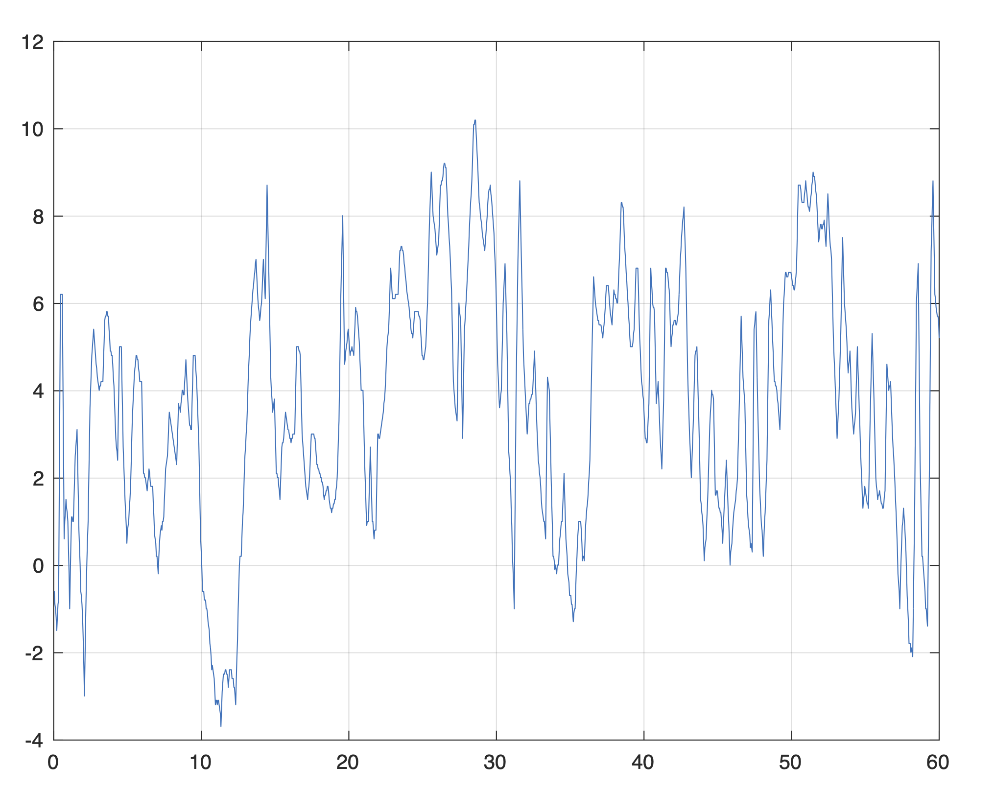
The issue is that, while the time constant of the system is of several days, a discretization of the system should be performed with a time step of one hour because of the fast variations of the outer temperature. This is the problem that we shall address in this paper.

Before going on, let us recall a result on differential equations.

Observe that we never use the differential formulation (6) of the ODE in the proof.

We use the previous lemma to estimate a kind of BIBO behavior using only the integral of the input.

2.4.1 Discussion

We consider a signal defined on an interval and split this interval into \( N\) consecutive intervals. On each interval we compute the average of the signal.

We show now that the upper bound of the function \( I[g]\) is small when \( N\) is big and \( g\) is bounded.

Thus we may define a small number \( \alpha\) that represents how close the signal \( g\) is closed to its averaged signal \( LP[g]\) :

2.5.1 Example 1

2.5.2 Example 2

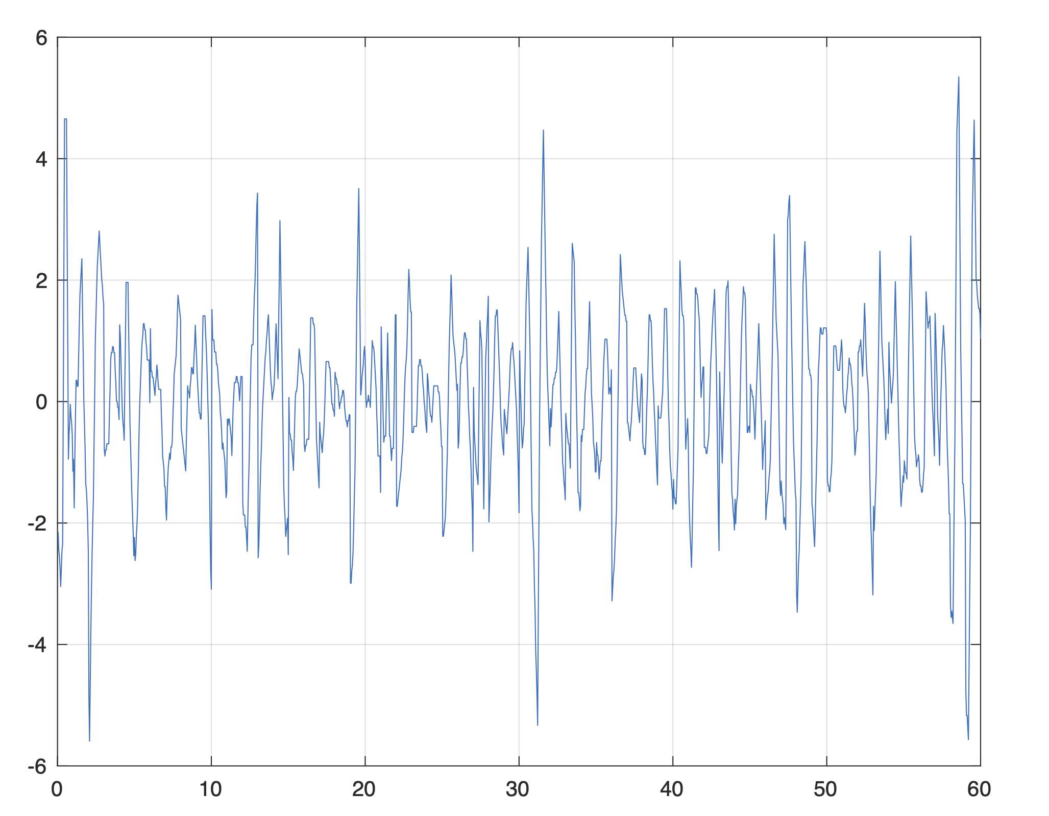
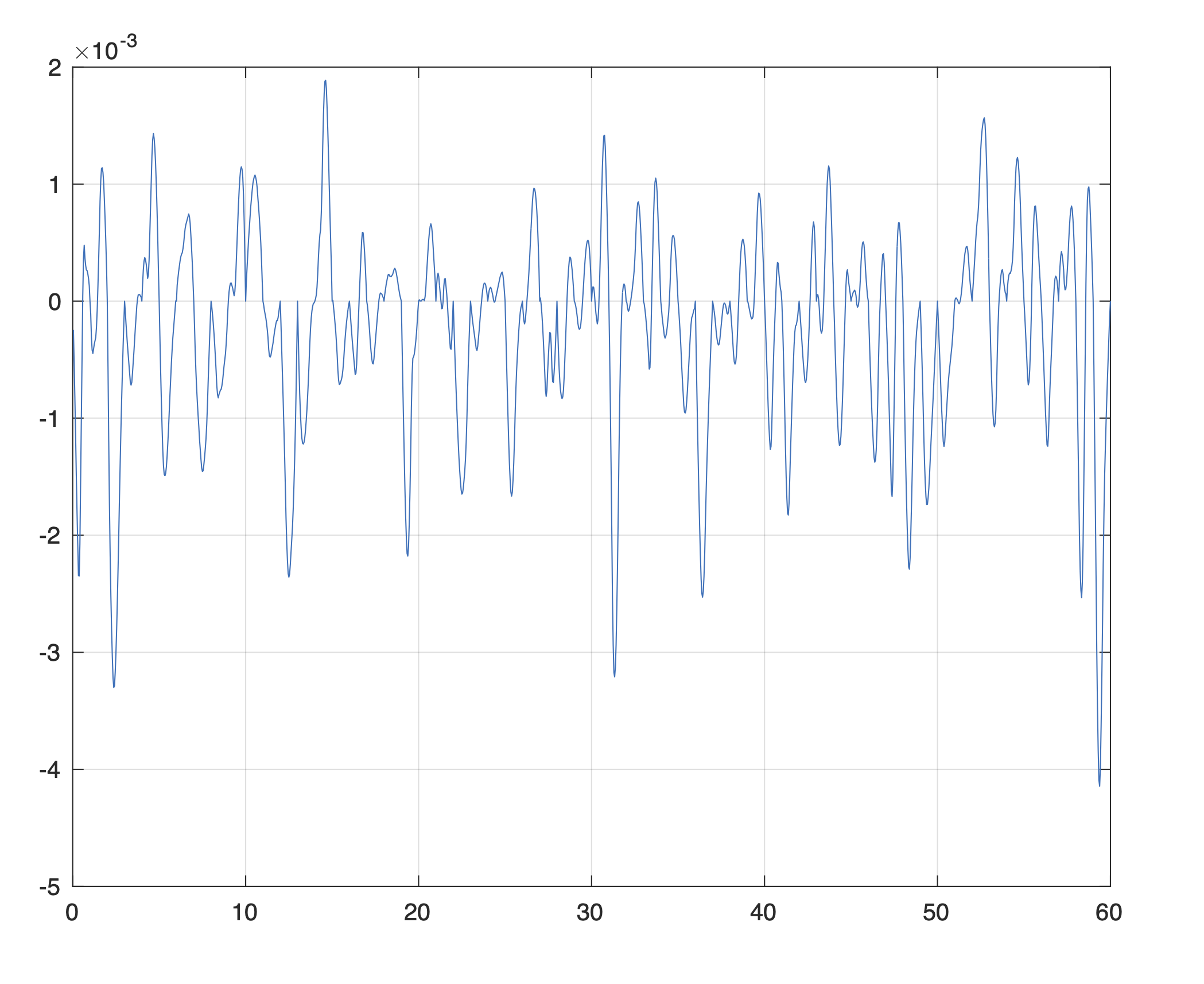
2.5.3 Application to the temperature signal

We use this averaging method on the temperature signal of figure 1 with an averaging window of 24 hours. Figure 2 shows the difference between the signal and its average; figure 3 shows the output of this difference through an integrator. Figure 3 indicates that the averaging error \( \alpha\) is much smaller than the sup norm obtained from figure 2.

Let us consider the ordinary differential equation (ODE):

with \( f\) Lipschitz with respect to \( x\) and integrable with respect to t.

The averaged ODE is defined as:

where the low-pass filter \( LP\) on a general function \( g(x,t)\) is defined as:

As a summary, \( LP[g]\) averages \( g\) with respect to time on rectangular adjacent windows, leaving the state variable unchanged.

The state \( x_{0}\) is well defined and bounded because \( f\) , and thus \( LP[f]\) , is Lipschitz.

We now estimate the distance between the trajectories obtained respectively from the nominal and averaged system.

In other words, the averaging error \( \|x-x_{0}\|_{\infty}\) is in first order in \( \alpha\) , that is small when \( N\) is big because \( f\) is Lipschitz and thus bounded on \( [0,T]\) .

If we want to have an a priori error estimate, i.e. an estimate that does not depend on the trajectory \( x_{0}\) , we can use an error bound linked to the difference between the vector fields.

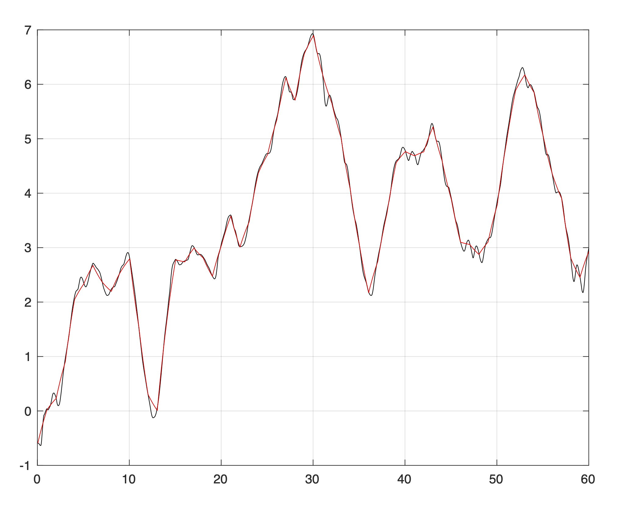
2.6.1 Application to the example system

Because the heating system is linear time invariant, we have \( \alpha = A\) . For the simulation we take a time constant of \( 3\) days = \( 72\) hours. Figure 4 displays the superposition of the inner temperature simulated with the original system (in black) and the averaged system (in red). For this system we have \( \alpha =0.2754\) , and the maximum error of the output temperature is \( 0.4613\) . Remember that the error estimate (26) is conservative since is does not take into account the stability of the system.

In the scope of this article, we define, for the integer \( N>0\) , and any functions \( u(t)\) and \( g(x,u(t),t)\) , an averaged function \( LP[g,u]\)

As a summary, \( LP[g]\) averages \( g\) with respect to time (this includes the open loop control) on rectangular adjacent windows, leaving the state (or costate) unchanged. The control is considered as an input signal among others.

We define the averaged OCP which consists in minimizing the cost

where \( y\) is the state defined by

The system (31) is a well defined differential equation.

The optimal trajectory \( x_{0}\) is defined by the ODE:

Since this is a new kind of optimal control, it is wise to study its stationarity condition.

We define an averaging error \( \alpha\) for the two point boundary value problem similarly to what was defined for initial boundary value problems.

For a function \( g(x,u,t)\) , the difference \( g(x_{0}(t),u_{0}(t),t)-LP]g,u_{0}](x_{0}(t),t)\) is the result of high pass filtering \( HP]g,u](x_{0}(t),t)\) . Let’s define the antiderivative:

Let’s define similarly the backwards antiderivative

We shall see that \( \alpha\) measures how close the nominal and averaged problems are. Observe that \( \alpha\) is small, for instance, when \( N\) is big and assumption 2 below holds (bounded functions and their derivatives).

Observe that that \( \alpha\) depends only on the solution of the averaged problem. It is an a posteriori estimate like in definition (25), and not an a priori estimate.

Technically, the proof of our main approximation result is based on the Pontryagin principle. This is a theoretical result which holds independently of the actual numerical method used to solve the nominal (resp. averaged) problem.

Now that we have stated what the averaged optimal control problem is, we can begin to evaluate its benefit when solving numerically a general optimal control problem.

Let us consider a direct method for the solving of problem (1,2). To do so, we discretize the dynamics into

In order to represent accurately the influence of the data on the system, the discretization step \( \delta t\) must be a suitable sampling rate for the data. In this article’s framework, \( \delta t\) is much smaller than the time constant of the system. The approximation of the cost is obtained by using a quadrature rule for the integral. Without using extra knowledge on the system, the time step of the quadrature is \( \delta t\) .

In this framework, the optimal control problem becomes a finite dimensional optimization problem with a finite number of equality constraints.

We consider now a similar direct method to solve the averaged problem (30,31). To avoid confusion, we denote by capital \( T_{K}\) the boundaries of the averaging intervals, and \( X_{K}\) denotes the state of the discretized averaged system. The dynamics of \( X\) is

where a suitable quadrature rule is used to compute the integral. Consistently with the discretization (39), we consider the sampling rate of the control and data to be \( \delta t\) . The computation of the cost is handled similarly.

We see that, while (39) only consider the differential aspect of the dynamics, the averaged dynamics (40) incorporates the integral action of a dynamical system.

Let us now consider the benefit of solving the averaged problem versus solving the nominal problem. To make things even simpler, let us use a Riemann integral for the computation of (40) and define

We assume that \( R\) is a (large) integer. Indeed, \( \delta t\) is dictated by the sampling rate of the data, while \( T_{K+1}-T_{K}\) is dictated by the time constant of the system, which is much larger.

We see that the number of control variables \( u_{k}\) is the same in both problems. However, the number of constraints (40) for the averaged problem is \( R\) times smaller than the number of constraints (39) for the original problem. This is the main benefit of using averaging to solve the optimal control problem with direct methods.

Finally, observe that the definition of the averaged costate (34) indicates what should be the two point boundary problem used in an indirect method for solving the averaged problem. In this case, the benefit of using the averaging method is a coarser grid for the two point boundary value problem.

In what follows we shall take great care to give explicit expressions for the various constants that are used throughout the article to obtain error bounds. This is not for the sake of displayed complicated expressions. This is for the following reason: the parameter \( \alpha\) , though very important in the scope of this work, is not the only one to influence the error bounds. Typically, the magnitude of the dynamics, cost, and their derivatives are also very important. In fact, if some part of the dynamics is large, this means that we are close to the situation where we want to use averaging while also having singular perturbations, and this a difficult framework to work with.

So yes, the details of the expressions are also important, and the tedious computations are necessary to obtain this kind of granularity in the expression of the final result. The homogeneity of the expressions of the bounds with respect to the numerical parameters of the various assumptions gives precious insight on their physical meaning.

where \( p\) is the costate of the nominal problem defined by the ODE with final condition:

The variable \( \alpha\) defined by the equation (38) is viewed as a small quantity Actually it is not required that \( \alpha\) be small. Its purpose is to give a one dimensional direction to a variation in a high dimensional space.. In Appendix B we compute a formal expansion of the state \( x\) and the costate \( p\) at the first order with respect to \( \alpha\) .

These formal expansions lead to the definition of auxiliary variables \( \tilde{x_{1}}\) and \( \tilde{p_{1}}\) as follows:

The error terms \( \tilde{x_{1}}\) and \( \tilde{p_{1}}\) correspond to the deviation error due to the approximation of the dynamics with respect to their fast oscillating behavior.

In definition 8 of section 4.3 we define deviations that are defined in magnitude, by contrast to the sole averaging error (at the optimum) which is considered here.

A consequence of the definition of \( \alpha \tilde{x_{1}}\) in definition 5 and \( \alpha\) in definition 2 is that:

And a consequence of the definition of \( \alpha \tilde{p_{1}}\) in definition(5) and \( \alpha\) in definition 2 is that:

We make two kinds of assumption on the problem data; the first is related to the regularity of the functions involved, and the second is a convexity assumption (Legendre-Clebsch) that is common in optimal control [24, 24, 6].

A consequence of that assumption is that the value \( \alpha\) defined by equation (38) is well defined and small if \( N\) is sufficiently big (or if the problem is periodic of small period).

As a consequence, we can bound the second derivative of the dynamics \( f\) :

Moreover, as \( p_{0}\) is the solution of the ODE with final condition (34), it is differentiable and thus continuous of the bounded interval \( [0,T]\) , so that it is bounded. So that another consequence of the assumption 2 involves the derivatives of the Hamiltonian:

As a consequence, the Hessian of the Hamiltonian is bounded:

The consequence of equation (47) is that \( H_{uu}\) is invertible and \( \|H_{uu}^{-1}\|_{\infty} \le \frac{1}{\beta} \) on any \( (x,u,p_{0})\) .

The consequence of equation (48) is :

where \( \tilde{x}_{1}\) and \( \tilde{p}_{1}\) are defined in definition 5 as the averaging errors on the dynamics of the optimal state and costate at the optimal solution of the averaged problem (as defined in section 2.8).

Moreover, we have:

Finally, we have:

The \( \delta\) variables are deviations in magnitude around the optimal control \( u_{0}\) , after a correction due to the pure averaging error on the various dynamics.

Here \( r\) and \( v\) are variations with respect to the solution of the averaged optimal control problem, with the extra corrective terms

• the averaging error on the optimal dynamics considered as a pure signal
• the correction term that corresponds to the second variation in reference [24], as defined in definition 6.

The quantity \( z^{2}\) is repeatedly used in [24] to study perturbations in optimal control; it has been used later in [27] in a similar manner.

We will bound \( \|r\|_{\infty}^{2}\) and \( \|v\|_{2}^{2}\) with respect to \( z^{2}\) and \( \alpha^{2}\) . Bounding then \( z^{2}\) with respect to \( \alpha^{2}\) will lead to the main result.

Let us recall we we stand in the expansion of the state and of the control. We have

We now define an extra correction term that will be used furter on. We will show that this correction term is also bounded by values that depend only on \( z\) and \( \alpha\) .

The state \( r_{1}\) is driven by the difference between the dynamics with state \( r_{1}\) and input \( v\) , and the nominal velocity of the system for the value of the state and controls that include all the previously introduced correction terms.

We will bound \( \|r-r_{1}\|_{\infty}\) in \( \alpha^{2}\) and \( \|r_{1}\|_{\infty}^{2}\) in \( z^{2}\) and \( \alpha^{2}\) . As a consequence, we will “anchor” our error estimates to the nominal term \( r_{1}\) .

This condition appears because \( \alpha\) is a numerical value determined by data, and not a parameter that tends to zero. In fact, the previous assumption is always satisfied if we can chose \( \alpha\) arbitrarily small.

To prove the main theorem, we proceed the following way.

The section 6.2 is devoted to the search of a lower bound of any real cost \( J(u)\) of the nominal problem. That lower bound contains two integral terms that do not depend on \( u\) , a term in \( z^{2}\) that is the only one depending on \( u\) , and a term in \( \alpha^{2}\) , that dos not depend on \( u\) either.

The section 6.3 is devoted to the search of an upper bound of the real cost \( J(u_{0})\) of the nominal problem controlled by \( u_{0}\) . That upper bound contains the same two integral terms as in the lower bound of \( J(u)\) and a term in \( \alpha^{2}\) .

Then the section 6.4.1 uses the assumption \( \alpha \leq \frac{\beta}{k_{J1}}\) to obtain a lower bound of \( J(u)\) independent of \( u\) , so that it is also a lower bound for \( J^{*}\) . That lower bound is combined with the upper bound of \( J(u_{0})\) to bound the suboptimality \( J(u_{0})-J^{*}\) as a function of \( \alpha^{2}\) , as stated in the equation (61) of the first part of the main theorem 3.

Then the section 6.4.1 uses the stronger assumption \( \alpha \leq \frac{\beta}{2k_{J1}}\) to obtain, for any \( u\) better than \( u_{0}\) , i.e. so that \( J(u) \leq J(u_{0})\) , an upper bound of \( z^{2}\) . With that bound of \( z^{2}\) , upper bounds for \( \|x-x_{0}\|_{\infty}\) and \( \|u-u_{0}\|_{2}\) are found in the equations (62) and (63) of the second part of the main theorem, with the help of the definitions and bounds of \( r\) and \( v\) in section 4.3.

6.2.1 Expansion of the real cost \( J(u)\)

6.2.2 Lower Bound of the third term of the expansion of \( J(u)\) in equation (64)

6.2.3 Lower Bound of the fourth term of the expansion of \( J(u)\) in equation (64)

6.2.4 Bound in absolute value for the sum of the integral terms of the right hand sides of equations (65) and (66)

6.2.5 Lower Bound of the real cost \( J(u)\)

As in the previous section, we first compute an expansion with integral remainder of the cost; then we study each term of the expansion to obtain a global bound in section 6.3.5.

6.3.1 Expansion of the cost \( J(u_{0})\)

6.3.2 Comparison of \( x^{0}\) and \( x_{0}\)

6.3.3 Upper Bound of the third term of the development of \( J(u_{0})\) (70)

6.3.4 Upper Bound of the fourth term of the development of \( J(u_{0})\) (70)

6.3.5 Upper Bound of \( J(u_{0})\)

The main theorem is proved in two steps. The first step compares the costs to estimate the suboptimality of the real system controlled by \( u_{0}\) . The second step compares the trajectories and controls which outperform \( u_{0}\) , to estimate how close they are from the trajectory and control driven by \( u_{0}\) .

6.4.1 Comparison of the real cost controlled by \( u_{0}\) and the infimum cost of the real system

6.4.2 Comparison of the controls and trajectories with and without \( u=u_{0}\)

Let \( u_{0}\) be the optimal control of the averaged problem (31) and let \( x_{0}\) be the corresponding trajectory. \( x_{0}\) is defined by the ODE with initial condition (32). Let \( p_{0}\) be the costate of the optimal trajectory, defined by the ODE with final condition (34), with \( H\) the hamiltonian (33).

The system constituted of the of equations (32) and (34) is a two boundaries problem. It is defined as the two boundaries problem corresponding to the averaged optimal control problem.

Let \( \delta u \in \mathbf{L}_{[0,T]}^2\) a scalar square integrable function on \( [0,T]\) .

Let \( \epsilon > 0\) and let \( u_{\epsilon} = u_{0} + \epsilon \delta u\) the variation of \( u_{0}\) in the direction of \( \delta u\) .

Since \( J_{0}(u_{0})=\min_{u}J_{0}(u)\) , the following stationarity condition holds:

Let \( x_{\epsilon}\) be the trajectory corresponding to \( u_{\epsilon}\) , defined by the dynamics equation 31 with \( v=u_{\epsilon}\) :

Let \( \delta x\) be the variation trajectory corresponding to the direction \( \delta u\) given by \( \delta x = \left(\frac{dx_{\epsilon}}{d \epsilon}\right)_{\epsilon =0}\) .

Let’s make use of Equation (78) in developing \( \left(\frac{dJ_{0}(u_{\epsilon})}{d \epsilon}\right)_{\epsilon=0}\) for a given \( \delta u\) .

Let’s now make use of equation (81). Let’s first fix \( t\) and let \( k\) be so that \( t \in [T_{k},t_{k+1})\) . Then we have:

Let’s specialize \( \delta u\) as a “needle variation”:

with \( \eta > 0\) so that \( t+\eta < t_{k+1}\) and \( \delta v \in \mathbf{L}_{[0,T]}^2\) .

Then we have:

More precisely, the limit is the value of the function at \( t\) everywhere the function is continue, that is for any \( t\) possibly except for a countable number of “jumps”. As any countable set is negligible, the limit holds almost everywhere.

Thus, because of the equations (78) and (81), we have:

and this is true for any \( \delta v \in \mathbf{L}_{[0,T]}^2\) . This proves the stationnarity result:

A.3.1 Remark

The state variable \( x\) is the solution of the original dynamics equation (2) driven by the control \( u\) . Let us define a formal expansion of \( x\) and \( u\) with regards to \( \alpha\) :

Note that the redundant definitions of \( x_{0}\) and \( u_{0}\) are consistent, as will be seen later.

We now separate the expansion terms \( x_{0}\) and \( x_{1}\) of the state into low (\( LP\) ) and high (\( HP\) ) frequencies components:

Because of the equations (83) and (85), and because the derivative of the high frequency signal \( \tilde{x_{1}}\) is in \( \frac{1}{\alpha}\) The integral of \( HP\) is in \( \alpha\) , so we consider that the derivative of \( HP\) is formally in \( \frac{1}{\alpha}\) , the derivative of \( x\) has the following expansion in \( \alpha\) :

But, because \( x\) is the solution of the original dynamics equation (2), using the formal expansions in \( \alpha\) of \( x\) and \( u\) , and thanks to assumption 2, we have another expansion of \( \frac{dx}{dt}\) at the first order in \( \alpha\) :

Consequently, identifying the zero order terms in equations (86) and (87), we obtain:

But by definition of \( \bar{x_{0}}\) as the low frequency part of \( x_{0}\) , we have:

Consequently, by definition of \( HP\) , we have:

with initial value \( 0\) . Integration the previous equation yields

But \( I[f,\bar{x_{0}},u_{0}]\) is of order 1 in \( \alpha\) and \( \tilde{x_{0}}\) is of order 0. Thus \( \tilde{x_{0}}=0\) , that gives \( x_{0}=\bar{x_{0}}\) the solution of the averaged problem. A consequence of that is that both definitions of \( x_{0}\) and \( u_{0}\) are consistent.

Moreover, we have a definition of \( \tilde{x_{1}}\) consistent with definition 5:

so that so that the derivative of \( \tilde{x_{1}}\) is \( -\frac{1}{\alpha}HP[f_{x},u_{0}](x_{0},p_{0},t)\) , that is in \( \frac{1}{\alpha}\) .

The costate variable \( p\) is the solution of the costate dynamics equation with ending condition (41). We expand it at the first order with respect to \( \alpha\) :

We then separate the expansion terms \( p_{0}\) and \( p_{1}\) into low (\( LP\) ) and high (\( HP\) ) frequencies components:

Because of the equations (88) and (89), and because the derivative of the high frequency signal \( \tilde{p_{1}}\) is in \( \frac{1}{\alpha}\) , the derivative of \( p\) has the following expansion in \( \alpha\) :

On the other hand, \( p\) is the solution of the costate dynamics equation with ending condition (41). Moreover, we have defined the developments in \( \alpha\) of \( x\) , \( p\) and \( u\) .

Thus we have another development of \( \frac{dp}{dt}\) at the first order in \( \alpha\) :

Consequently, identifying the zero order terms in equations (90) and (91), we have:

But by definition of \( \bar{p_{0}}\) as the low frequency part of \( p_{0}\) , we have:

Consequently, by definition of \( HP\) , we have:

with final value \( 0\) . Integration of the previous equation yields

But \( I[-H_{x},x_{0},p_{0},u_{0}]\) is of order 1 in \( \alpha\) as \( \tilde{p_{0}}\) is of order 0. Thus \( \tilde{p_{0}}=0\) , that gives \( p_{0}=\bar{p_{0}}\) , the solution of the averaged costate equation. A consequence of that is that both definitions of \( p_{0}\) are consistent.

Moreover, we have a definition of \( \tilde{p_{1}}\) consistent with definition 5:

so that the derivative of \( \tilde{p_{1}}\) is \( -\frac{1}{\alpha}HP[H_{x},u_{0}](x_{0},p_{0},t)\) , that is in \( \frac{1}{\alpha}\) .

Proposition 12 is important since it bounds \( r\) and \( v\) with respect to \( z\) and \( \alpha\) . To obtain a bound on \( r\) and \( v\) which only depends on \( \alpha\) , it will be enough to provide a bound of \( z\) involving \( \alpha\) only.

D.1.1 Upper bound for \( r\)

D.1.2 Upper bound for \( v\)

We now turn our attention to the variable \( r\) , which can be approximated by the variable \( r_{1}\) , up to an error which is bounded by a term that depends only on \( z\) and \( \alpha\) .

The variable \( r\) follows the dynamic (96) with \( r(0)=0\) , and \( r_{1}\) follows the dynamic (58).

Thus \( r-r_{1}\) follows the dynamics:

Thus, in a similar way than for the upper bound of \( r\) , the following inequality holds:

The equation (59) follows from Gronwall lemma.

The equation (60) is then the consequence of equations (56) and (59), together with:

The remaining appendix sections are devoted to the obtention of a lower bound on \( J(u)\) . This is achieved by obtaining a lower bound on each term of the expansion (64) of \( J(u)\) . Only the complicated terms require an extensive study; this study is detailed in sections F, G, H and finally I.

[1] J.A. Sanders and F. Verhulst Averaging Methods in Nonlinear Dynamical Systems Springer-Verlag 1985

[2] H. Poincaré Les méthodes nouvelles de la mécanique céleste Gauthier-Villars 1892

[3] V. I. Arnold Mathematical Methods of Classical Mechanics Springer-Verlag 1978

[4] V. I. Arnold Geometrical Methods in the Theory o f Ordinary Differential Equations Springer-Verlag 1983

[5] M. Balachandra An Averaging Theorem for Two-Point Boundary Value Problems with Applications to Optimal Control Journal of Mathematical Analysis and Applications 1976 55 46-60 10.1016/0022-247X(76)90277-8

[6] François Chaplais Averaging and Deterministic Optimal Control SIAM Journal on Control and Optimization 1986 25 3 767-780 May 10.1137/0325044

[7] E. N. Barron Averaging In Lagrange And Minimax Problems Of Optimal Control SIAM Journal on Control and Optimization 1993 31 6 1630-1652 November 10.1137/0331077

[8] Vladimir Gaitsgory and Sergey Rossomakhine Occupational Measures Formulation And Linear Programming Solution Of Deterministic Long Run Average Problems Of Optimal Control Proceedings of the 45th IEEE Conference on Decision and Control 2006 5012-5017 10.1109/CDC.2006.377568

[9] Vladimir Gaitsgory and Sergey Rossomakhine Linear Programming Approach To Deterministic Long Run Average Problems Of Optimal Control SIAM Journal on Control and Optimization 2006 44 6 2006–2037 10.1137/040616802

[10] Luke Finlay and Vladimir Gaitsgory and Ivan Lebedev Duality In Linear Programming Problems Related To Deterministic Long Run Average Problems Of Optimal Control SIAM Journal on Control and Optimization 2008 47 4 1667–1700 10.1137/060676398

[11] Luke Finlay and Vladimir Gaitsgory and Ivan Lebedev Duality in Linear Programming Problems Related to Deterministic Long Run Average Problems of Optimal Control with Applications to Periodic Optimization Proc. of the Joint 48th IEEE Conference on Decision and Control and 28th Chinese Control Conference 2009 1207-1211 10.1109/CDC.2009.5400261

[12] A. P. Ogulenko and O. D. Kichmarenko Averaging of the Problem of Optimal Control on Time Scales Journal of Mathematical Sciences 2016 212 3 290-304 January 10.1007/s10958-015-2665-1

[13] Jean-Baptiste Caillau Bernard Bonnard and Romain Dujol Energy minimization of single input orbit transfer by averaging and continuation Bull. Sci. math. 2006 130 707–719 10.1016/j.bulsci.2006.03.005

[14] Jean-Baptiste Caillau Bernard Bonnard and Romain Dujol Averaging and optimal control of elliptic Keplerian orbits with low propulsion Systems and Control Letters 2006 55 755–760 10.1016/j.sysconle.2006.03.004

[15] Bernard Bonnard and Jean-Baptiste Caillau Riemannian metric of the averaged energy minimization problem in orbital transfer with low thrust Ann. Inst. H. Poincaré, Analyse non linéaire 2007 24 395–411 10.1016/j.anihpc.2006.03.013

[16] Sophie Geffroy and Richard Epenoy Optimal Low-Thrust Transfers With Constraints-Generalization Of Averaging Techniques Acta Astronautica 1997 41 3 133-149 10.1016/S0094-5765(97)00208-7

[17] Ch. Ferrier and R. Epenoy Optimal Control for Engines with Electro-Ionic Propulsion Under Constraint of Eclipse Acta Astronautica 2001 48 4 181–192 10.1016/S0094-5765(00)00158-2

[18] M. Robillart and P. Schalbart and F. Chaplais and B. Peuportier Model reduction and model predictive control of energy-efficient buildings for electrical heating load shifting Journal of Process Control 2019 74 23-34 10.1016/j.jprocont.2018.03.007

[19] Christophe Coudurier and Olivier Lepreux and Nicolas Petit Optimal bang-bang control of a mechanical double oscillator using averaging methods 9th IFAC Vienna International Confererence on Mathematical Modelling, MATHMOD 2018 2018 10.1016/j.ifacol.2018.03.009

[20] Onésimo Hernández-Lerma and Jean B. Lasserre Average cost optimal policies for Markov control processes with Borel state space and unbounded costs Systems and Control Letters 1990 15 349-356 10.1016/0167-6911(90)90108-7

[21] Alessandro N. Vargas and João B. R. do Val Average optimal stationary policies: convexity and convergence conditions in linear stochastic control systems Proc. of the joint 48th IEEE Conference on Decision and Control and 28th Chinese Control Conference 2009 3388-3393 10.1109/CDC.2009.5400501

[22] Ching-Chih Tsai and Abraham H. Haddad Averaging, Aggregation And Optimal Control Of Stochastic Hybrid Systems With Singularly Perturbed Morkovian Switching Behavior Proceedings of the American Conference 1994 1994 1868-1872

[23] R. Buckdahn, M. Quincampoix, J. Renault On representation formulas for long run averaging optimal control problem Journal of Differential Equtaions 2015 259 5554–5581 10.1016/j.jde.2015.06.039

[24]

[25] Panagiotis Tsiotras and François Chaplais and Dongwon Jung Redundant wavelet processing on the half-axis with applications to signal denoising with small delays: Theory and experiments International Journal on Adaptive Control and Signal Processing 2006 20 9 447 - 474 10.1002/acs.911

[26] Somaya Goumri Transfert orbital d'un engin a faible poussee MINES ParisTech 2015

[27] D. Maamria and F. Chaplais and A. Sciarretta and N. Petit Impact of regular perturbations in input constrained optimal control problems Optimal Control, Applications and Methods 2020 41 4 1321-1351 July 10.1002/oca.2605